728x90
반응형
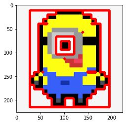
#cv2.boundingRect(contour): Contour를 포함하는 사각형을 그립니다.
#사각형의 X, Y 좌표와 너비, 높이를 반환합니다.
import cv2
import matplotlib.pyplot as plt
image = cv2.imread('image_5.png')
image_gray = cv2.cvtColor(image, cv2.COLOR_BGR2GRAY)
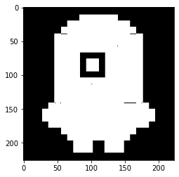
ret, thresh = cv2.threshold(image_gray, 230, 255, 0)
#논리곱(bitwise_and), 논리합(bitwise_or), 배타적 논리합(bitwise_xor), 부정(bitwise_not)
#검,흰을 단절하기 위해
thresh = cv2.bitwise_not(thresh)
plt.imshow(cv2.cvtColor(thresh, cv2.COLOR_GRAY2RGB))
plt.show()
contours = cv2.findContours(thresh, cv2.RETR_TREE, cv2.CHAIN_APPROX_SIMPLE)[0]
image = cv2.drawContours(image, contours, -1, (0, 0, 255), 4)
plt.imshow(cv2.cvtColor(image, cv2.COLOR_BGR2RGB))
plt.show()
contour = contours[0]
x, y, w, h = cv2.boundingRect(contour)
image = cv2.rectangle(image, (x, y), (x + w, y + h), (0, 0, 255), 3)
plt.imshow(cv2.cvtColor(image, cv2.COLOR_BGR2RGB))
plt.show()

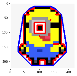
#cv2.convexHull(contour): Convex Hull 알고리즘으로 외곽을 구하는 함수
#대략적인 형태의 Contour 외곽을 빠르게 구할 수 있습니다. (단일 Contour 반환)

import cv2
import matplotlib.pyplot as plt

image = cv2.imread('image_5.png')
image_gray = cv2.cvtColor(image, cv2.COLOR_BGR2GRAY)
ret, thresh = cv2.threshold(image_gray, 230, 255, 0)
thresh = cv2.bitwise_not(thresh)

contours = cv2.findContours(thresh, cv2.RETR_TREE, cv2.CHAIN_APPROX_SIMPLE)[0]
image = cv2.drawContours(image, contours, -1, (0, 0, 255), 4)

plt.imshow(cv2.cvtColor(image, cv2.COLOR_BGR2RGB))
plt.show()

contour = contours[0]
hull = cv2.convexHull(contour)
image = cv2.drawContours(image, [hull], -1, (255, 0, 0), 4)

plt.imshow(cv2.cvtColor(image, cv2.COLOR_BGR2RGB))
plt.show()

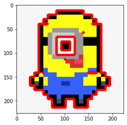
#cv2.approxPolyDP(curve, epsilon, closed): 근사치 Contour를 구합니다.

#curve: Contour
#epsilon: 최대 거리 (클수록 Point 개수 감소)
#closed: 폐곡선 여부

import cv2
import matplotlib.pyplot as plt

image = cv2.imread('image_5.png')
image_gray = cv2.cvtColor(image, cv2.COLOR_BGR2GRAY)
ret, thresh = cv2.threshold(image_gray, 230, 255, 0)
thresh = cv2.bitwise_not(thresh)

contours = cv2.findContours(thresh, cv2.RETR_TREE, cv2.CHAIN_APPROX_SIMPLE)[0]
image = cv2.drawContours(image, contours, -1, (0, 0, 255), 4)

plt.imshow(cv2.cvtColor(image, cv2.COLOR_BGR2RGB))
plt.show()

contour = contours[0]
epsilon = 0.01 * cv2.arcLength(contour, True)
approx = cv2.approxPolyDP(contour, epsilon, True)
image = cv2.drawContours(image, [approx], -1, (0, 255, 0), 4)

plt.imshow(cv2.cvtColor(image, cv2.COLOR_BGR2RGB))
plt.show()


#cv2.contourArea(contour): Contour의 면적을 구합니다.
#cv2.arcLength(contour): Contour의 둘레를 구합니다.
#cv2.moments(contour): Contour의 특징을 추출합니다.

import cv2
import matplotlib.pyplot as plt

image = cv2.imread('image_5.png')
image_gray = cv2.cvtColor(image, cv2.COLOR_BGR2GRAY)
ret, thresh = cv2.threshold(image_gray, 230, 255, 0)
thresh = cv2.bitwise_not(thresh)

contours = cv2.findContours(thresh, cv2.RETR_TREE, cv2.CHAIN_APPROX_SIMPLE)[0]
image = cv2.drawContours(image, contours, -1, (0, 0, 255), 4)

contour = contours[0]
area = cv2.contourArea(contour)
print(area)

length = cv2.arcLength(contour, True)
print(length)

M = cv2.moments(contour)
print(M)

plt.imshow(cv2.cvtColor(image, cv2.COLOR_BGR2RGB))
plt.show()
24290.0
762.2842707633972
{'m00': 24290.0, 'm10': 2696190.0, 'm01': 2724271.0, 'm20': 333820896.0, 'm11': 302394081.0, 'm02': 373703711.3333333, 'm30': 44722844388.0, 'm21': 37604953834.0, 'm12': 41481111958.0, 'm03': 57020772797.5, 'mu20': 34543806.0, 'mu11': 0.0, 'mu02': 68160175.66264582, 'mu30': 0.0, 'mu21': 164913234.29575968, 'mu12': 1.9073486328125e-06, 'mu03': -181522929.26306152, 'nu20': 0.058548416866933635, 'nu11': 0.0, 'nu02': 0.11552491866182932, 'nu30': 0.0, 'nu21': 0.0017934394646650165, 'nu12': 2.0742509390277333e-17, 'nu03': -0.001974070707376463}
728x90
반응형
'Data Analysis > Data Analysis & Image Processing' 카테고리의 다른 글
| 13. KNN Algorithm (0) | 2022.04.16 |
|---|---|
| 12. OpenCV Filtering (0) | 2022.04.16 |
| 10. OpenCV Contours (0) | 2022.04.16 |
| 9. OpenCV 도형 그리기 (0) | 2022.04.16 |
| 8. OpenCV Tracker (0) | 2022.04.16 |


댓글